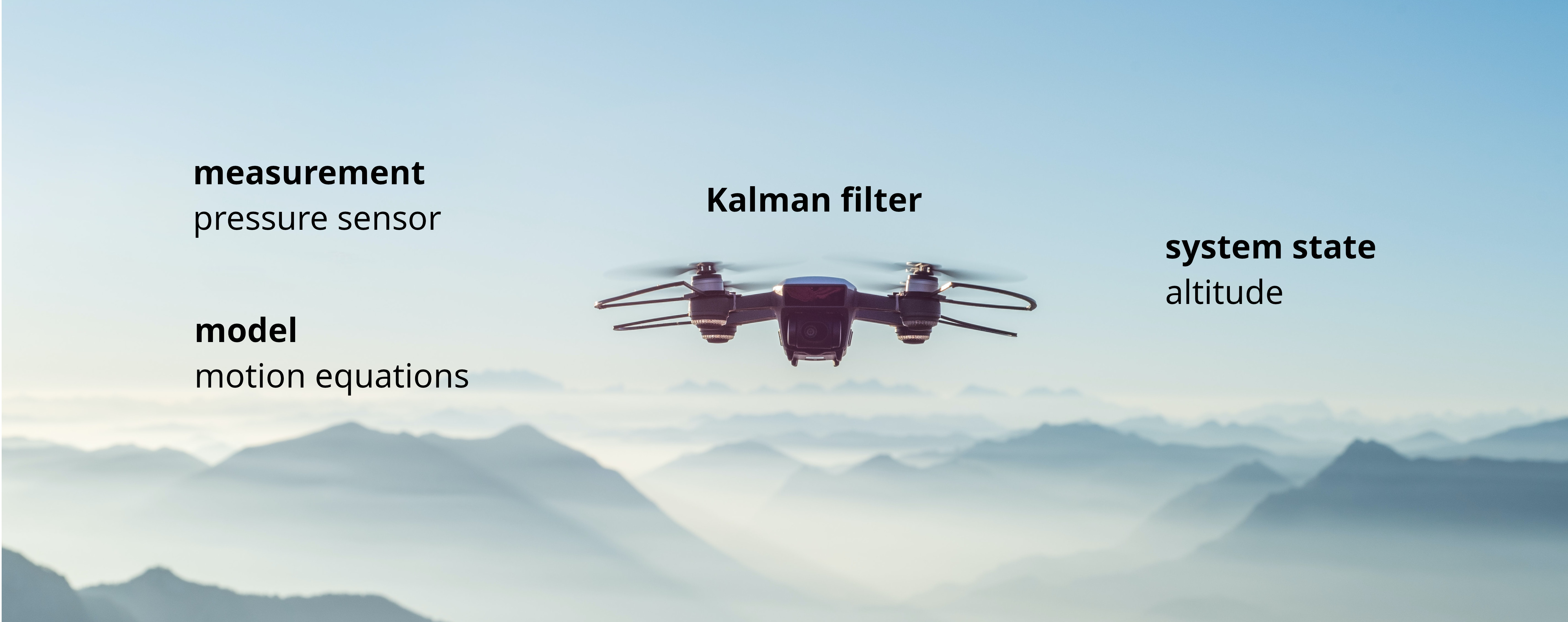
Let’s say we want to know the altitude of the drone we are flying. On one hand, our drone has a pressure sensor that allows us to measure the altitude. On the other hand, we know the altitude of the drone a second ago and the thrust produced by propellers, so the current altitude can be calculated from it. The question is how to combine these data to get one more accurate result, and often the answer is to use a Kalman filter. Kalman filter can provide an optimal estimate given a model and a measurement in the form of a normal (aka Gaussian) distribution. In this article, I will try to explain why normal distribution works and how it gives Kalman filter its superpower.
Accepting the uncertainty
As you most certainly know, the world isn’t perfect. Every time you measure something, you never get the true value because every measuring device has an uncertainty that defines its quality. One of the most common ways to define the measuring uncertainty is to use a plus-minus sign. We could say that the drone is flying at 15 ± 5 m above the ground. What does this say about the true value of the altitude? It can be either 12, 19, 15, or 13.486. All of these values are equally likely. In probability theory, this case is described by a uniform distribution.
With the uniform distribution, it is quite easy to calculate the probability that a random variable equals any particular value inside the uncertainty range (±5 in our case). For example, the probability of the true value of the altitude to be 16 m:
\[P(X = 16) = {1 \over {b - a}} = {1 \over {5 - (-5)}} = 0.1 = 10\%\]At the same time, for all the values outside of our uncertainty range, the probability equals zero.
The drawback of the uniform distribution is that it can’t represent measurement uncertainty. If the sensor gives the value of 12 m you expect it to be close to this value. In other words, it is common to think that the value of 11.99 m is much more likely than the value of 10 m even knowing that the measurement uncertainty of the device is 2 m. One way to model this situation is to switch to a normal distribution.
Why normal distribution?
Why not any other non-uniform distribution? The main reason for that is the central limit theorem. It states that “when independent random variables are added, their properly normalized sum tends toward a normal distribution (informally a “bell curve”) even if the original variables themselves are not normally distributed” [wiki].
To confirm this fact, let’s use a coin flip simulation. The experiment consists in the following. We toss a coin 20 times and write down the number of heads which can go from 0 to 20. Then we repeat the experiment 50 or 5000 times. When running the experiment 50 times it is difficult to see any pattern. However, after 5000 tries we see that the graph starts to look like a bell curve which can be closely approximated by Gaussian distribution. As you’ve already guessed, this is one of the reasons why we assume normal distribution in the Kalman filter.
Properties of normal distribution
Another nice fact about normal distribution is that we need only two variables to define it: mean \(\mu\) and variance \(\sigma^2\). The notation is the following:
\[X \sim \mathcal{N}(\mu,\,\sigma^{2})\]which says that some random variable \(X\) follows a normal distribution with mean \(\mu\) and variance \(\sigma^2\).
However, to extract the probability we have to use a probability density function (PDF). And in the case of Gaussian, it has the following form:
\[\begin{equation} \label{gaussiandistrib} \begin{aligned} f(x) = \frac{1}{\sigma\sqrt{2 \pi}}e^{ - {1\over{2}} \left ( \frac{x-\mu}{\sigma} \right )^2} \end{aligned} \end{equation}\]One of the important properties of this function is that the total area under the curve is equal to 1. In other words, we are 100% sure that the random variable \(X\) will take the value from the range \((-\infty,\infty)\); something will happen, we guarantee. Could we do better than that? What is the probability of one exact value?
To find the probability from the probability density function, we need to find the area under the curve in the given range. In the case of one particular value, the width of the range equals zero, so the probability is also zero. It means that we can only estimate the probability in a range: \(P(x_1 < X \leq x_2)\).
Some interesting properties of the normal distribution:
- the probability density function is symmetric around the mean
- the probability of a variable to be in the range of \([\mu-3\sigma,\mu+3\sigma]\) is 99.73%
- the probability of a variable to be in the range of \([\mu-2\sigma,\mu+2\sigma]\) is 95.45%
- the probability of a variable to be in the range of \([\mu-\sigma,\mu+\sigma]\) is 68.27%
- the probability of a variable to be in the range of \((-\infty,\mu]\) or \((\mu,\infty)\) is 50.00%
Multiple measurements
Now, let’s get back to the Kalman filter and the drone example. The altitude given by our pressure sensor can be modeled as a normal distribution \(\color{#ff8000}{\mathcal{N}_{s} (\mu_{s}, \sigma_{s}^2 )}\) with \(s\) for sensor; it also can be calculated given motion equations that define the model \(\color{royalblue}{\mathcal{N}_{m} (\mu_{m}, \sigma_{m}^2 )}\). These distributions represent probability distributions and to combine them, we need to use the probability rule of product:
\[\begin{equation} \label{fusionformula_1} \begin{aligned} P &= \color{royalblue}{\mathcal{N}_{m} (\mu_{m}, \sigma_{m}^2 )} \cdot \color{#ff8000}{\mathcal{N}_{s} (\mu_{s}, \sigma_{s}^2 )}\\ &= \mathcal{N} (\mu, \sigma^2 ) \end{aligned} \end{equation}\]with
\[\begin{equation} \label{fusionformularearranged} \begin{aligned} \mu &= \frac{\sigma_s^2 \mu_m + \sigma_m^2 \mu_s} {\sigma_m^2 + \sigma_s^2}\\ \sigma &= \frac{\sigma_m^2 \sigma_s^2} {\sigma_m^2 + \sigma_s^2} \end{aligned} \end{equation}\]Let’s use the following graph to get the intuition behind these expressions:
| \(\color{royalblue}{\mathcal{N}_{m}}\) | \(\color{#ff8000}{\mathcal{N}_{s}}\) | \(\color{royalblue}{\mathcal{N}_{m}} \cdot \color{#ff8000}{\mathcal{N}_{s}}\) |
|---|---|---|
| \(\color{royalblue}{\mu_m} =\) | \(\color{#ff8000}{\mu_s} =\) | \(\mu =\) |
| \(\color{royalblue}{\sigma_m} =\) | \(\color{#ff8000}{\sigma_s} =\) | \(\sigma =\) |
Note that:
- the resulting distribution is also a normal distribution
- the mean of the new resulting distribution is located always “in between” the two initial means and closer to the distribution with lower variance (lower uncertainty). The lower the variance, the more we “trust” the given source of the information.
- it has a variance smaller than each individual variance of the measurement or the model. Given more sources of information, we become more and more certain about the state of our system, the altitude of the drone
While in the example above we have only one variable, the Kalman filter often works with systems defined by many variables. Multidimensional Kalman filter involves some linear algebra but the main principle stays the same: get the information from different sources in the form of a normal distribution and then combine it to get a result with higher certainty/smaller variance.
KEY TAKEAWAYS
- Kalman filter allows combining multiple sources of information about the system to provide an optimal estimate of the system state.
- Each piece of information needs to be presented in the form of a normal distribution defined by a mean and a variance.
- A product of two normal distributions is also a normal distribution with smaller variance.